
The Flaw of Averages — Comparing Monte Carlo Simulations with Estimates based on Averages

Some weeks ago, my boss challenged me: Why do we need to run those 10'000 simulations when doing Monte Carlo forecasts? Could we not use the average throughput and get the same result? While he was not rejecting my arguments, he pushed me to prove it with data: Are Monte Carlo Simulations really performing better or is it just the assumption?
Let’s run an experiment and see what the data has to say, shall we?
Note: This post was originally published on Medium in the Mastering Agility publication.

In this post, I share a comparison of the two approaches:
Forecast how many items will be done using Monte Carlo Simulations
Estimate how many items will be done using the average throughput
I’ll be using real data from one of the teams I’m working with, so it’s not a theoretical exercise but one that is based on a real team with all the variability like sick leaves, vacation days, and interruptions.

The Flaw of Averages
First, let’s quickly summarize what the supposed problem with using averages is. I can recommend diving deeper into this topic, either by reading the book “The Flaw of Averages” by Sam Savage or by watching Prateek Singh and Dan Vacanti talk about it on Drunk Agile.
The Flaw of Averages: Why We Underestimate Risk in the ...
Read 39 reviews from the world's largest community for readers. A must-read for anyone who makes business decisions…www.goodreads.com
In a nutshell, using averages is problematic because:
It is heavily affected by outliers and it is impacted vastly by the data sample
It assumes that the underlying process can be represented by a normal distribution. This is a problem because, in non-normal distribution the mean (average) and the median can be vastly different, bringing inaccurate results when used for forecasting
In short, plans based on average, fail on average. Two examples to show the flaw of averages:
If Bill Gates walks into a bar, on average everyone in the bar will be a millionaire
If you roll two six-sided dice, the most likely (average) result will be a 7. However, the chance to get a 7 will only be 16.666%. Even though it’s the most likely result, it’s not very likely.
The Seven Deadly Sins of Averaging
In his book "The Flaw of Averages" Sam Savage identifies seven (now eleven) deadly sins of averaging. How many of these…www.linkedin.com
But enough with the theory, let’s see what the data says. That’s why we’re here after all.
Sample Data
Before we look at the forecasts, let's look at where we get our data from.
Team
For this analysis, we look at a team that has 6 developers and works on a single product. The team has been working in this configuration for the last few months, so it’s reasonable to assume that the future performance of the team will look like the past few weeks.
History
We will look at a 28-day history of this team. We’ll be using the teams' throughput from the 1st to the 28th of October. In this period, the team managed to close 35 items overall.
The team is pretty predictable, as you can see in their throughput per week (the October timespan is indicated with the red lines):

We can also look at the throughput run chart per day. You can see that the team manages to close items on a regular basis and does not batch-closing items too much (for example, there is no “last day of the Sprint” where suddenly all items get closed):

This data is the base for both, the calculation using the average throughput as well as for the Monte Carlo Simulation.
Running the Forecasts
Now that we have our context, we’ll be running our forecasts. We want to forecast the next 30 days, so how many items can we close between the 29th of October and the 27th of November? We’ll use both the average as well as the Monte Carlo forecast.
Forecast using Average
Let’s first use the average. We closed 35 items in 28 days. Thus we would get an average of 1.25 items per day:
35 items / 28 days = 1.25 items/day
As we want to forecast the next 30 days, we can now simply calculate:
1.25 items/day * 30 days = 37.5 items
Seems reasonable, let’s see what our Monte Carlo Simulation was saying before we look at the real number of items closed.
Forecast using Monte Carlo Simulation
We’re running every night new forecasts for various “configurations” (for example different spans of historical data that should be taken into account).
The Full Monte
Just how accurate are Monte Carlo forecasts for software development teams?medium.com
On the 28th of October, our forecast that used the past 28 days as input forecasted the following for the next 30 days:
50% probability of closing 38 items or more
70% probability of closing 35 items or more
85% probability of closing 31 items or more
95% probability of closing 27 items or more
Interim Analysis
Before we look at the real number of closed items, I think it’s interesting to point out that Monte Carlo Simulations give you more than one result, and you can choose the “risk profile” that you feel fits best to your environment. This is important, as it will give you some context to the number.

If we look at the calculation with the average, we see it might be quite risky, at least according to our MC forecast. This tells us that we only have a 50% chance of achieving this number. It still happens one out of two times, but when using the average, you are missing this detail. “There is a 50% chance we manage 38 items” is different information than “we manage 38 items”.
But now let’s look at how the team did perform in real life the next 30 days.
Reality
So in reality, from the 29th of October till 27th of November, we managed to close…30 items!
You can see in the throughput chart, that it dropped a bit over this period:

If we look at the per-day throughput, we can see that there were no periods of no items being done (so no days where nobody was working except weekends):

So it seems no special things happened, just some variability in the throughput from the team.
Interpreting the Data
Below is a summary of our data. You can see that the forecast based on the average was quite far off, while the 85th percentile of the Monte Carlo Simulation was quite close to the real result:
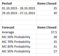
I think we can see here, that using an average of the throughput for forecasts is flawed. Not only was it quite far off from the real number, but using an average you also get a sense of “certainty”. It’s a single number, with no probability attached to it.
On the other hand, Monte Carlo Simulations give you proper forecasts with a “risk” attached to them. You can be more risky and go for the number that only half of the simulations managed to achieve. But it’s a well-informed decision you are taking.

Conclusion
While we aim for predictability, we’ll most likely never get rid of all variability in our process. And as long as we have variability, the Monte Carlo Simulations will perform better. We’ll make the uncertainty visible by having different “risk profiles” with each forecast, which allows us to make more informed decisions. Using an average is not only performing worse, you also pretend to have an “exact number”.
Using Monte Carlo forecasts, continuously updating them, and inspecting the results is the best way of reducing risk. I highly recommend using them with your teams over averages or other methods of estimation you might use at the moment.